How Qwen3.5 works

Qwen3.5 connects a vision encoder that accepts dynamic resolutions to a hybrid language backbone. Images and videos become visual tokens in the same sequence as text. The language layers alternate between Gated DeltaNet and Full Attention, processing context through recurrent matrix states and a history of keys and values, respectively.

This article follows Qwen3.5-9B through preprocessing, visual encoding, multimodal fusion, and language computation, with comparisons to 4B Dense and 35B-A3B MoE. The emphasis is on tensor shapes, state update equations, and the connections between modules. The derivations are included because they help explain what the implementation actually does.

Configuration values come from the official checkpoints. The source links identify one consistent implementation. The equations and simplified code explain its execution; parameter and cache sizes are analytical calculations, not measurements of throughput, peak memory, or model quality. The diagrams follow the same configurations and computational relationships.

1. Overall architecture: one visual front end, two token mixers

1.1 The overall computation

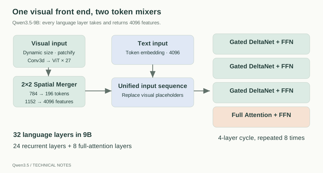
Qwen3.5-9B converts images and videos into visual tokens, substitutes them for visual placeholders in the input sequence, and passes the result to an autoregressive language backbone. Its 32 language layers follow a repeating pattern of three Gated DeltaNet layers and one Full Attention layer, giving 24 of the former and 8 of the latter. S1, S2, C1

image / video                        text / chat template
      |                                       |
resize + normalize + patchify          tokenization
      |                                       |
pixel_values + grid_thw         input_ids + modality types
      |                                       |
Vision Transformer                    token embedding
      |
2x2 spatial merger ----------------> placeholder replacement
                                              |
                                multimodal input embeddings
                                              |
                    [ Gated DeltaNet + Dense SwiGLU ] x 3
                    [ Full Attention + Dense SwiGLU ] x 1
                                   repeat 8 times
                                              |
                                      RMSNorm + LM head
                                              |
                                   next-token distribution

The multipliers describe the arrangement of layer types. Every layer has its own parameters and state. A single DeltaNet module is not run three times with shared weights, and a router does not choose the attention type for each token. S1

Dense versus MoE and linear versus full attention describe separate parts of a layer. The first distinction concerns the FFN and its use of sparse experts; the second concerns how tokens exchange information. A dense 9B model can therefore have a hybrid attention stack, while the token mixer in the 35B-A3B MoE model remains separate from its expert FFN. S1, S9

1.2 The checkpoint configuration

These values come from the 9B checkpoint, rather than the defaults obtained by constructing a configuration class without arguments. C1

Subsystem	Qwen3.5-9B configuration
Text hidden size / number of layers	4096 / 32
Dense FFN intermediate size	12288
Full Attention	16 Q heads, 4 KV heads, head dimension 256
Gated DeltaNet	16 Q/K heads, 32 V heads, K/V head dimensions both 128
DeltaNet local convolution	Depthwise causal Conv1d, kernel=4
Vocabulary / configured context length	248320 / 262144
Text RoPE	theta=10000000; partial factor=0.25; sections=[11,11,10]
Vision encoder	27 layers, width 1152, 16 heads, FFN width 4304
Visual patches	Spatial size 16×16, temporal size 2, spatial merger 2×2
Learned visual position table	2304 positions, a 48×48 grid
Visual merger output size	4096, matching the language backbone
Embedding and LM head	Untied weights

max_position_embeddings=262144 is a configuration value. It does not mean every machine can run that context length efficiently, nor does it guarantee equal quality under arbitrary lengths, position changes, or extended generation. Section 13 calculates the KV cache cost alone.

1.3 Changing model size involves more than hidden_size

Configuration	4B Dense	9B Dense	35B-A3B MoE
Text width	2560	4096	2048
Text layers	32	32	40
Full Attention Q/KV heads	16 / 4	16 / 4	16 / 2
Full Attention head dimension	256	256	256
Dense FFN intermediate size	9216	12288	Not applicable
Routed experts / experts selected per token	Not applicable	Not applicable	256 / 8
Expert / shared expert intermediate size	Not applicable	Not applicable	512 / 512
Vision depth / width	24 / 1024	27 / 1152	27 / 1152
Vision output size	2560	4096	2048
Tied token embedding and LM head	Yes	No	No

Sources: C1, C4, C5. These three checkpoints share the same DeltaNet head configuration. That observation should not be generalized to every future model in the family.

The 4B model illustrates a useful trap: its text width is 2560, but the total Q width inside Full Attention is 16×256=4096. Read the explicit head_dim and projection definitions instead of assuming head_dim = hidden_size / num_heads.

2. Modules and their source files

The outer model has the following structure. S1

Qwen3_5ForConditionalGeneration
  model: Qwen3_5Model
    visual: Qwen3_5VisionModel
      patch_embed
      pos_embed
      rotary_pos_emb
      blocks[0:27]
      merger
    language_model: Qwen3_5TextModel
      embed_tokens
      layers[0:32]
        input_layernorm
        linear_attn OR self_attn
        post_attention_layernorm
        mlp
      norm
      rotary_emb
  lm_head

Start with modeling_qwen3_5.py, where the executed logic is expanded. Then consult modular_qwen3_5.py for inheritance relationships. Several definitions in the modular file inherit or reuse implementations, so a pass statement alone tells little about the full behavior. The generated file’s header also specifies that upstream changes belong in the modular file, from which the modeling file is generated. S1, S3

Preprocessing is spread across more than the qwen3_5/ directory. The 9B processor configuration reuses Qwen3VLProcessor, the image path reuses the Qwen2-VL implementation, and the video path reuses the Qwen3-VL implementation. Reusing a code class does not imply that the model reuses all the earlier model’s weights or architecture. S4, S5, S6, C2

3. Notation: three different sequence lengths

Let $F$ be the number of sampled frames and $H\times W$ the spatial size after resizing. The spatial patch size is $p=16$, the temporal patch size is $\tau=2$, and the spatial merge factor is $m=2$.

After any necessary padding by repeating the final frame:

$$T_g=\left\lceil\frac{F}{\tau}\right\rceil, \qquad H_g=H/p,\qquad W_g=W/p.$$

A still image is repeated along the temporal axis to provide two frames, producing one temporal group, so $T_g=1$. All spatial dimensions used below are assumed to be aligned to $pm=32$. S4, S5

The three lengths are:

$$N_{\rm patch}=T_gH_gW_g, \qquad N_{\rm vis}=\frac{T_gH_gW_g}{m^2}, \qquad L=N_{\rm text/special}+N_{\rm vis}.$$

N_patch is the ViT input length. N_vis is the number of merged visual tokens that occupy positions in the language sequence. L also includes the chat template, timestamps, boundary markers, question, and other text tokens. The two visual lengths differ by a factor of four and cannot be used interchangeably. Text length must come from tokenization, not a character count.

The second dimension of pixel_values, 1536, is the raw pixel feature size of one patch. It is distinct from both the ViT hidden size and the LLM hidden size.

4. Image preprocessing: from pixels to ordered patches

4.1 Read the checkpoint’s preprocessing parameters

The Qwen3.5-9B image processor uses patch_size=16, temporal_patch_size=2, and merge_size=2, with image_mean=image_std=0.5 for all three channels. Its saved processor type includes the name Qwen2VLImageProcessorFast; that name does not imply a patch size of 14. C2

For ordinary uint8 RGB pixels, with rescaling and normalization enabled:

$$x_{\rm norm}=\frac{x/255-0.5}{0.5}=\frac{x}{127.5}-1.$$

If an external loader has already converted the image to floating-point values in $[0,1]$, check whether rescaling should be disabled. Dividing by 255 twice changes the input distribution. RGB conversion, sampling, resizing, and normalization are all part of the input protocol; matching the final tensor shape is insufficient. S4

4.2 How smart_resize works

The spatial alignment factor is:

$$f=p\times m=32.$$

smart_resize first rounds height and width to multiples of this factor, then checks the area budget. If the area is too large, it uses the original height and width to compute:

$$\gamma=\sqrt{HW/P_{\max}},\qquad H'=f\left\lfloor\frac{H/\gamma}{f}\right\rfloor, \qquad W'=f\left\lfloor\frac{W/\gamma}{f}\right\rfloor.$$

If the area is too small, the corresponding operation enlarges the image and rounds upward. The implementation also checks extreme aspect ratios. This keeps the grid aligned and the area within budget while retaining the aspect ratio as closely as possible. Images are not simply forced into a fixed square. S4

On this execution path, the 9B configuration values size.shortest_edge=65536 and size.longest_edge=16777216 are used as pixel area limits, despite their names. They correspond to merged image token budgets of 64 and 16384. Aspect ratio, rounding, and user overrides still determine the actual shape. C2, S4

For an aligned image that requires no further resizing:

$$N_{\rm vis}=\frac{HW}{(pm)^2}=\frac{HW}{1024}.$$

The visual token count therefore changes with the input resolution.

4.3 Why a still image needs temporal_patch_size=2

The visual patch embedding uses a 3D convolution with a temporal extent of two frames. For a still image, the processor repeats the same spatial pixels at both temporal positions. The inspected image implementation can do this at patch level with unsqueeze + expand; it need not first materialize an entire two-frame video. S4

Repeating pixels adds no motion information. It gives images and videos compatible tubelet inputs:

$$D_{\rm raw}=C\tau p^2=3\times2\times16^2=1536.$$

4.4 Patch order is more than row-major flattening

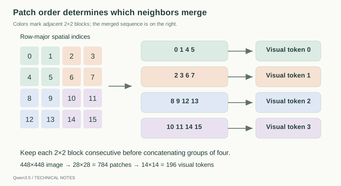
A 448×448 image has $H_g=W_g=28$. For the later view(-1, 4D_v) to merge adjacent patches correctly, the processor places the four patches of each 2×2 spatial block next to each other. S4

The shape changes can be illustrated as follows:

[B, 3, 448, 448]
  -> [B, 3, 14, 2, 16, 14, 2, 16]
  -> [B, 14, 14, 2, 2, 3, 16, 16]
  -> insert / repeat temporal dimension of size 2
  -> [B, 784, 1536]
  -> concatenate images in their original order
  -> [sum_of_raw_patches, 1536]

Consider a 4×4 patch grid with ordinary row-major indices:

 0  1  2  3
 4  5  6  7
 8  9 10 11
12 13 14 15

The block-major order required by the merger is:

[0, 1, 4, 5,  2, 3, 6, 7,
 8, 9, 12, 13,  10, 11, 14, 15]

Patch order, position-coordinate order, and the merger reshape must stay consistent. Together they determine which image region each visual token represents; changing any one requires checking the other two.

4.5 Image processor outputs

For one 448×448 image:

image_grid_thw = [[1, 28, 28]]
pixel_values.shape = [784, 1536]
number_of_image_placeholders = 784 / 4 = 196

Images of different sizes are grouped by shape for efficient processing, then restored to their original order. The final pixel_values is usually a concatenation with variable total length. It need not be a padded batch of shape [B, N, 1536]. S4

5. Video preprocessing: sampling, temporal grouping, and timestamps

5.1 Sampled frames and temporal groups

The inspected video processor supports sampling by target fps or by num_frames; callers cannot explicitly set both. With fps sampling, it estimates a frame count from the original frame count and fps, applies minimum and maximum constraints, then selects uniformly spaced frame indices. S5

There are three separate quantities. Original frame indices determine physical time. The order of sampled frames determines the input content. Pairs of sampled frames form temporal groups and determine the temporal length of the visual grid. A 30fps source, 2fps target sampling rate, and temporal patch size of 2 do not give the model 30 independent visual blocks per second.

For an odd number of sampled frames, patchification repeats the last frame, giving $T_g=\lceil F/2\rceil$. Using $F//2$ for every input would undercount these groups.

5.2 The video pixel budget includes time

The video version of smart_resize checks a total pixel count approximately equal to $FHW$. It changes spatial dimensions; it does not resample the temporal axis inside this function. S5

The 9B video configuration specifies size.longest_edge=25165824 and shortest_edge=4096. With an even frame count, ideal alignment, and no additional per-frame cap, the budget gives:

$$N_{\rm vis}=\frac{FHW}{2\times32^2} \lesssim\frac{25165824}{2048}=12288.$$

This explains the configuration’s budget. It does not guarantee that every processed video has exactly 12288 tokens. C3, S5

The implementation also exposes cap_pixels_per_frame. When enabled, it applies an additional per-frame pixel limit and budget allocation rules. When unspecified, it retains the uncapped behavior and warns about a future default change. A statement from an older utility package such as “at most 768 tokens per frame” is therefore not a universal guarantee. Reproducible experiments should record whether loading went through qwen-vl-utils, the processor budgets, sampling parameters, and this switch. S5

5.3 Video patch order

For eight frames of size 448×448:

input video:       [B, 8, 3, 448, 448]
temporal grouping: [B, 4, 2, 3, 14, 2, 16, 14, 2, 16]
permute:           [B, 4, 14, 14, 2, 2, 3, 2, 16, 16]
flatten:           [B, 3136, 1536]
public output:     [sum_of_raw_video_patches, 1536]
video_grid_thw:    [[4, 28, 28]]

The permutation corresponds to (0,1,4,7,5,8,3,2,6,9) in the source. It packs matching spatial patches from two frames into a tubelet and places adjacent tubelets from each 2×2 spatial block together. S5

At the processor output, video_grid_thw is organized per video, with shape [num_videos,3]. Expanding temporal blocks for MRoPE happens later.

5.4 Timestamps for temporal groups

Suppose the source runs at 30fps and the sampled original frame indices are explicitly given as:

[0, 15, 30, 45, 60, 75, 90, 105]

Their times are 0, 0.5, 1.0, 1.5, 2.0, 2.5, 3.0, and 3.5 seconds. With temporal_patch_size=2, the processor groups pairs and takes the average of each group’s first and last timestamps:

[0.25, 1.25, 2.25, 3.25] seconds

The source formats each timestamp to one decimal place and follows it with a visual segment. S6

<0.2 seconds><|vision_start|>[196 video tokens]<|vision_end|>
<1.2 seconds><|vision_start|>[196 video tokens]<|vision_end|>
<2.2 seconds><|vision_start|>[196 video tokens]<|vision_end|>
<3.2 seconds><|vision_start|>[196 video tokens]<|vision_end|>

[196 video tokens] is explanatory shorthand, not a literal string to pass to the tokenizer.

Three details matter here. A group timestamp is not the time of its second frame and need not be an integer number of seconds. The tokenizer further splits timestamp text, so <0.2 seconds> should not be counted as a single token. Finally, externally sampled video needs its real frames_indices and source fps preserved. If metadata is absent, the source may fall back to 24fps, producing a valid shape with incorrect temporal meaning. S6

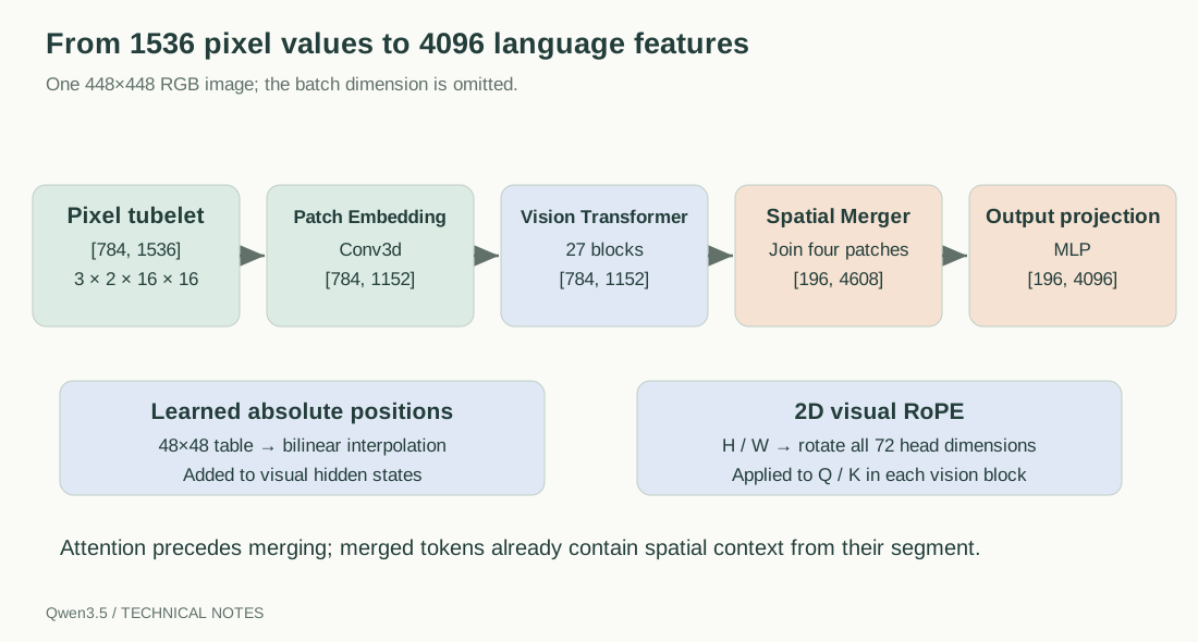
6. The vision encoder: from 1536 pixel values to language features

6.1 Patch embedding applies Conv3d to packed patches

In 9B, Qwen3_5VisionPatchEmbed uses kernel and stride [2,16,16], with 3 input channels and 1152 output channels. S1

[784, 1536]
   -> view [784, 3, 2, 16, 16]
   -> Conv3d
   -> [784, 1152, 1, 1, 1]
   -> view [784, 1152]

Within this call, each already packed tubelet is one input item and produces one embedding. This step fuses local information across two frames. It does not give the entire ViT global attention across all video times.

6.2 Learned absolute positions and bilinear interpolation

The learned visual position table has shape [2304,1152], corresponding to a 48×48 base grid. An input grid may instead be 28×28 or 44×80, so the table cannot simply be added as a fixed-length sequence. S1, C1

The implementation uses bilinear interpolation with align_corners=True. Target row $r$ maps to the following row coordinate in the base table:

$$u=r\frac{48-1}{H_g-1}.$$

The column mapping is analogous. With fractional parts $a,b$ along the two axes, the interpolated vector is a weighted sum of the four neighboring embeddings:

$$E(u,v)=(1-a)(1-b)E_{00}+(1-a)bE_{01} +a(1-b)E_{10}+abE_{11}.$$

The implementation then rearranges positions into the same spatial block order as patchification and repeats them across temporal groups. These embeddings provide a two-dimensional positional prior on the model’s input grid. They do not directly encode physical world coordinates from the original image. S7

6.3 Visual RoPE rotates the full head in two spatial dimensions

The 9B vision head dimension is $1152/16=72$. Its rotary module uses H and W axes. Each axis supplies 18 frequencies; concatenating them gives 36, which are duplicated according to the rotate_half layout to cover 72 dimensions:

vision spatial coordinates: [N_patch, 2]
H frequencies:              [N_patch, 18]
W frequencies:              [N_patch, 18]
concatenated frequencies:   [N_patch, 36]
cos / sin after duplication:[N_patch, 72]

The Q/K rotation can be written as:

$$q'=q\odot\cos\phi+\operatorname{rotate\_half}(q)\odot\sin\phi.$$

Visual RoPE rotates the full 72-dimensional head. The language Full Attention layers discussed later rotate only 64 dimensions of a 256-dimensional head. S1

Learned absolute position embeddings are added to hidden states, while RoPE acts on Q/K inside each attention layer. These are separate ways of introducing position information, rather than two applications of the same position vector.

6.4 Vision attention is standard noncausal multihead attention

Each vision block applies LayerNorm, attention, and a residual addition, followed by another LayerNorm, a two-layer GELU MLP, and another residual addition. S1

$$X'=X+\operatorname{Attn}(\operatorname{LN}(X)), \qquad X''=X'+\operatorname{MLP}(\operatorname{LN}(X')).$$

For a 448×448 image, the QKV shapes are:

hidden states: [784, 1152]
fused QKV:     [784, 3456]
reshape:       [784, 3, 16, 72]
Q, K, V each: [784, 16, 72]
backend form:  [1, 16, 784, 72]

qkv = Linear(1152, 3×1152) is a fused projection. Q, K, and V remain different vectors, and individual heads use different projection channels. Vision blocks set is_causal=False, allowing bidirectional interaction between spatial patches within the same attention segment. S1

The visual MLP is:

$$\operatorname{MLP}_{\rm vision}(x)=W_2\operatorname{GELU}(W_1x+b_1)+b_2,$$

with dimensions $1152\to4304\to1152$ in 9B and the configured gelu_pytorch_tanh activation. This differs from the language FFN’s SwiGLU. S1, C1

6.5 What cu_seqlens separates

The helper used by the Qwen3.5 vision path defaults to merge_temporal=False. Its logic is equivalent to:

lengths = repeat_interleave(grid_h * grid_w, grid_t)
cu_seqlens = [0] + cumsum(lengths)

An eight-frame, 448×448 video has four temporal groups, each containing 784 raw patches:

cu_seqlens = [0, 784, 1568, 2352, 3136]

Vision attention therefore consists of four bidirectional 784×784 blocks. It does not form a single block spanning all 3136 patches. Flash Attention uses variable-length sequence boundaries; other paths split the tensor according to these lengths and compute attention separately. S1, S7

The tubelet Conv3d performs local fusion across two frames. Longer-range interaction across temporal groups is handled mainly by the later language backbone. Video input alone is not evidence that the vision encoder uses full spatiotemporal attention.

6.6 What the spatial merger changes

The final merger receives [N_patch,1152]. On the main path it normalizes each patch, then uses the block-major order to concatenate groups of four:

[N_patch, 1152]
   -> LayerNorm(1152)
   -> [N_patch / 4, 4608]
   -> Linear(4608, 4608) + GELU
   -> Linear(4608, 4096)
   -> [N_vis, 4096]

Concatenation reduces the token count; the MLP learns the spatial merge and maps features to the language width. This operation is neither simple average pooling nor a width expansion that leaves sequence length unchanged. S1

A merged token also contains more than its nominal 32×32 pixel region. Before merging, ViT attention has already mixed information from other spatial positions within the same temporal group.

6.7 Return values and DeepStack

The inspected Qwen3_5VisionModel returns:

last_hidden_state: [N_patch, 1152]   # unmerged
pooler_output:    [N_patch/4, 4096] # merged

The return type is BaseModelOutputWithPooling. The outer get_image_features splits pooler_output into a tuple using the merged token count of each image. S1

This path has no three-group DeepStack feature output from Qwen3-VL, nor any extra injection from intermediate vision layers into language layers 0, 1, and 2. The 9B configuration has deepstack_visual_indexes=[], and the execution code lacks that branch. Adding visual features at multiple language depths would require an implementation change. S1, C1

7. Multimodal fusion: writing visual features into the language sequence

7.1 Expanding a placeholder into visual tokens

The chat template typically starts with:

<|vision_start|><|image_pad|><|vision_end|>

Before tokenization, the processor expands the image placeholder to $T_gH_gW_g/m^2$ image tokens. For video, it inserts a timestamp and visual segment for each temporal group. S6, C6

The model first embeds all input_ids, then replaces positions corresponding to <|image_pad|> or <|video_pad|> with merger features. A simplified version is:

inputs_embeds = token_embedding(input_ids)   # [B, L, D]
features = vision_encoder(pixels).pooler_output
features = features.to(inputs_embeds.device, inputs_embeds.dtype)
mask = (input_ids == image_token_id).unsqueeze(-1)
inputs_embeds = inputs_embeds.masked_scatter(mask, features)

The implementation checks that placeholder counts and feature element counts match. Each position in 9B needs exactly 4096 feature dimensions. Truncating a 3584-dimensional vector or calling .to() cannot make it a valid 4096-dimensional feature. S1

7.2 mm_token_type_ids is part of the position protocol

By default, the inspected processor returns mm_token_type_ids with the same length as input_ids: 0 for text, 1 for images, and 2 for video. Qwen3.5 uses these values to identify contiguous modality segments and construct MRoPE positions. S1, S6

On this path, the field does not index an additional modality embedding table, and it is not itself a causal mask. Position construction raises an error when multimodal grids are present but the type markers are missing. A custom collator or forward wrapper must retain this field.

7.3 One fused sequence

After replacement, text and visual tokens are vectors in the same [B,L,D] tensor and pass through the same decoder layers. The standard path has no separate cross-attention module at every layer that queries visual memory from text. Further visual interaction occurs through the token mixers of this unified sequence. S1

Visual tokens consequently update DeltaNet states and enter Full Attention K/V caches. Their cost in the language backbone persists after image encoding has finished.

8. The shared language decoder structure

8.1 Token mixing followed by an FFN

Whether a layer uses Gated DeltaNet or Full Attention, the 9B residual structure is:

$$U=X+\operatorname{Mixer}(\operatorname{RMSNorm}(X)),$$ $$Y=U+\operatorname{SwiGLU}(\operatorname{RMSNorm}(U)).$$

Both mixers accept and return [B,L,4096], allowing them to alternate within one stack. In a linear-attention layer, DeltaNet occupies the mixer position that Full Attention occupies elsewhere. S1

At initialization, config.layer_types[layer_idx] determines the layer type. With zero-based indexing, layers 0, 1, and 2 are linear and layer 3 is full attention; the pattern repeats through layer 31.

8.2 Zero-centered RMSNorm parameters

The text backbone and Q/K norms use a zero-centered parameterization, with trainable scale 1 + weight:

$$\operatorname{RMSNorm}(x)= \frac{x}{\sqrt{\operatorname{mean}(x^2)+\epsilon}} \odot(1+w).$$

The parameter $w$ starts at 0, so the effective initial scale is 1. The source computes normalization and scaling in float32, then restores the input dtype. S1

This does not initialize the output to zero. The 1 + weight convention matters when inspecting a state dict, porting a norm, or converting weights. DeltaNet’s output RMSNormGated uses a different implementation: its scale is initialized to 1 directly, and it applies a SiLU gate after normalization.

8.3 Dense SwiGLU

The 9B FFN computes:

$$\operatorname{SwiGLU}(x) =W_{\rm down}\left[\operatorname{SiLU}(W_{\rm gate}x) \odot(W_{\rm up}x)\right].$$

input:     [B, L, 4096]
gate/up:   [B, L, 12288] each
multiply:  [B, L, 12288]
down:      [B, L, 4096]

All three projections omit biases. Although their names share the word “gate,” the FFN gate, DeltaNet’s forgetting/write/readout gates, and Full Attention’s output gate belong to different modules and have different functions. S1

9. Gated DeltaNet: reading and writing a fixed-size matrix state

9.1 From stored K/V to a matrix state

Ordinary autoregressive attention retains the K/V of individual past tokens and lets each new query interact explicitly with those positions. Gated DeltaNet instead maintains one matrix per head. It decays this state, corrects the association addressed by the current key, and reads the result from the updated matrix. S1, P1

The delta rule determines how this works. It subtracts what memory already predicts for the current key, then writes the remaining error. Removing softmax or reordering a $QK^T$ multiplication alone does not produce this update.

The derivation below follows the source’s state orientation:

$$S_t\in\mathbb R^{d_k\times d_v}.$$

Keys and queries are $d_k$-dimensional column vectors, values are $d_v$-dimensional column vectors, and $S_t^Tk_t$ reads a value. Some papers transpose the state convention. Their equations can look reversed while describing the same operation.

9.1.1 How a fixed matrix can accumulate history

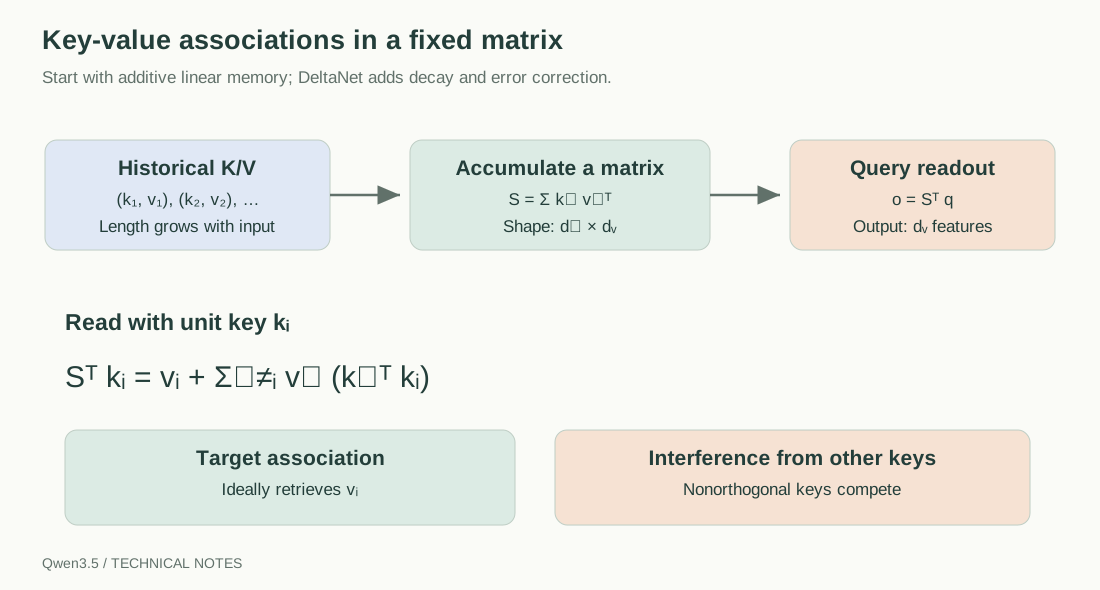
First set aside softmax, normalization, forgetting, and delta correction. A basic linear associative read for query $t$ is:

$$o_t=\sum_{j\le t}(q_t^Tk_j)v_j.$$

Here $q_t^Tk_j$ is a scalar measuring the match between the current query and key $j$. Since it is scalar:

$$(q_t^Tk_j)v_j=(v_jk_j^T)q_t.$$

Reassociating the sum gives:

$$o_t= \left(\sum_{j\le t}v_jk_j^T\right)q_t.$$

Using the state orientation $S_t\in\mathbb R^{d_k\times d_v}$ adopted here:

$$S_t=\sum_{j\le t}k_jv_j^T, \qquad o_t=S_t^Tq_t.$$

The mathematical step is reassociation. Instead of repeatedly reading a list whose length grows with $L$, the model can accumulate historical key/value associations into a $d_k\times d_v$ matrix. “Linear” here primarily refers to processing sequence length $L$ recurrently. Each step still performs matrix-state work involving $d_kd_v$; the entire model has not become a single linear layer.

This also clarifies the transpose. A column $k_j$ and a row $v_j^T$ form an outer product of shape $d_k\times d_v$. The value $v_j$ has not changed its meaning when written as the row $v_j^T$. If another paper defines its state as $\sum_jv_jk_j^T$, its read becomes $S_tq_t$, the transposed convention of the same construction.

9.1.2 The matrix as associative KV memory

After one write $S=kv^T$, querying with the same unit key gives:

$$S^Tk=(kv^T)^Tk=v(k^Tk)=v.$$

The key $k$ can be viewed as an address direction and the value $v$ as the content that should be returned along that direction. After several writes:

$$S=\sum_jk_jv_j^T,$$

querying with $k_i$ yields:

$$S^Tk_i =v_i+\sum_{j\ne i}v_j(k_j^Tk_i),$$

The first term is the requested value; the second is interference from other, nonorthogonal keys. A finite matrix is therefore not a lossless lookup table. Similar keys compete for nearby directions, and more writes can create collisions. A simple additive linear-attention state keeps adding $kv^T$. The delta rule first reads what the current key already retrieves, then writes only the prediction error, reducing the direct accumulation of repeated associations. P1

9.2 Six signals and the actual 9B dimensions

The normalized input hidden states have shape [B,L,4096]. The source has four projections, for QKV, z, b, and a. Splitting QKV gives six logical signals in total. S1

Signal	Projected width	Purpose
Q	16×128=2048	Read information from the state
K	16×128=2048	Address the association to write or correct
V	32×128=4096	Target content for the current write
z	32×128=4096	Gate each output element
b	32	Produce a write rate beta for each V head
a	32	Produce a state decay for each V head

The implementation uses in_proj_qkv: 4096→8192, then splits the result. Separate linear layers produce z, b, and a. These projections have no biases, but the decay equation includes a separate trainable dt_bias. S1

9.3 The causal depthwise convolution on Q/K/V

Projected QKV is arranged as [B,8192,L], passed through a causal Conv1d with kernel size 4 and groups=8192, then through SiLU. Each projected channel is convolved over nearby sequence positions independently; the convolution does not mix channels. S1

For channel $c$, an illustrative expression is:

$$u_{t,c}=\operatorname{SiLU}\left( \sum_{j=0}^{3}a_{c,j}\,r_{t-j,c}\right),$$

where missing left context is zero and the kernel indexing is pedagogical notation.

The convolution adds recent local context to Q/K/V. Its time axis is the order of the fused token sequence, which may include text, image patches, timestamps, and video patches. Four positions do not necessarily correspond to four physical video frames. The z, a, and b projections bypass this QKV convolution. S1

9.4 Q/K normalization and head expansion

After convolution, Q and K each have shape [B,L,16,128], while V has shape [B,L,32,128]. The source applies repeat_interleave(2) to the Q/K heads to match the 32 V heads. Every state corresponds to a V head, so there are 32 state heads, not 16. S1

The kernel call sets use_qk_l2norm_in_kernel=True, giving normalization of the form:

$$\bar k=\frac{k}{\sqrt{\sum_i k_i^2+\epsilon}}, \qquad \bar q=\frac{q}{\sqrt{\sum_i q_i^2+\epsilon}}.$$

The query also receives a $1/\sqrt{d_k}$ scale. This is different from the learned RMSNorm used by Full Attention. There is no basis here for inserting ELU, softmax, or a positive feature map from some other linear-attention method. S1

Below, $k_t$ denotes the L2-normalized key and $\tilde q_t=\bar q_t/\sqrt{d_k}$ denotes the final read query.

In 9B, every expanded head maintains:

$$S_t^{(h)}\in\mathbb R^{128\times128}.$$

Across the batch and 32 heads, the recurrent state is [B,32,128,128]. There is no length dimension $L$: one DeltaNet layer has the same matrix-state shape after 100 or 100000 tokens. History can still grow in the Full Attention KV caches elsewhere in the hybrid stack, so this property applies to the DeltaNet state, not to the model’s entire cache.

9.5 Three gates with different roles

The write gate for each V head is:

$$\beta_t=\sigma(b_t).$$

The log-decay is:

$$g_t=-\exp(A_{\log})\operatorname{softplus}(a_t+d_{\rm bias}).$$

The retention factor actually multiplied into the state is:

$$\alpha_t=\exp(g_t).$$

In real arithmetic, $\beta_t\in(0,1)$ and $\alpha_t\in(0,1)$. Finite precision can introduce saturation or underflow. The source explicitly computes decay in float32 to reduce numerical problems. S1

$\alpha$ determines how much of the old state survives. $\beta$ determines how much prediction error is corrected along the current key. The z signal determines which output channels are passed onward. Forgetting, writing, and output gating are separate operations.

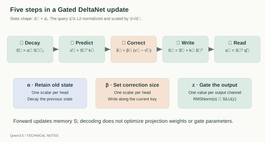
9.6 Deriving the recurrence from the source

First decay the previous state:

$$\bar S_t=\alpha_t S_{t-1}.$$

Use the current key to read a prediction from the decayed state:

$$\hat v_t=\bar S_t^T k_t.$$

Compute the difference between the target value and that prediction, scaled by the write rate:

$$\delta_t=\beta_t(v_t-\hat v_t).$$

Write the correction along the key direction:

$$S_t=\bar S_t+k_t\delta_t^T.$$

Finally, read the updated state with the query:

$$o_t=S_t^T\tilde q_t.$$

This follows the order in torch_recurrent_gated_delta_rule: decay, predict, correct, then read. Combining the steps gives:

$$S_t=\alpha_t(I-\beta_t k_tk_t^T)S_{t-1} +\beta_t k_tv_t^T.$$

The term $I-\beta_tk_tk_t^T$ distinguishes this update from a simple additive memory. S1

9.7 Why this is a delta rule

Treat the decayed state as the starting point and consider the local association error:

$$\ell(S)=\frac12\|S^Tk_t-v_t\|_2^2.$$

Its gradient is:

$$\nabla_S\ell=k_t(S^Tk_t-v_t)^T.$$

One gradient-descent step on this error with step size $\beta_t$ gives exactly the state correction above. This provides a mathematical interpretation of the delta rule.

The object being updated is the forward-pass memory state $S$. The projection weights and gate parameters remain model parameters. This operation is not an optimizer.step on the pretrained model during inference; state and parameters have different roles in the computation graph.

For that reason, $S_t$ is often called fast-weight memory. It changes at every token during the forward pass but is not permanently written back to the checkpoint by an optimizer. The “online gradient step” is an equivalent mathematical view of the state update. It does not require inference-time backpropagation, parameter gradient storage, or an optimizer.

If $k_t$ has exactly unit norm and $\beta_t=1$, the updated state can match the current value along the current key direction. It does not overwrite the whole matrix. Other directions can retain information, and different keys can still interfere. Actual L2 normalization includes epsilon, so the equality is an idealized explanation.

9.8 A 2×2 example by hand

Use idealized gate values to make the arithmetic transparent. The endpoints 0 and 1 are conceptual choices; this example does not claim that finite sigmoid inputs produce those exact endpoints.

Start with $S_0=0$. For $k_1=(1,0)^T$, $v_1=(2,0)^T$, and $\alpha_1=\beta_1=1$:

$$S_1=\begin{bmatrix}2&0\\0&0\end{bmatrix}.$$

On the second step, keep the same key but change the target value to $(0,4)^T$, with $\alpha_2=0.5$ and $\beta_2=0.5$:

$$\bar S_2=\begin{bmatrix}1&0\\0&0\end{bmatrix}, \quad \hat v_2=(1,0)^T,\quad \delta_2=(-0.5,2)^T.$$

The updated state is:

$$S_2=\begin{bmatrix}0.5&2\\0&0\end{bmatrix}.$$

For query $(1,0)^T$, including the $1/\sqrt2$ query scale, the readout is:

$$o_2=(0.353553\ldots,\ 1.414214\ldots)^T.$$

The old association first decays and then moves toward the new target. The update does not unconditionally add the new value to the old one.

9.9 Normalizing and gating the readout

Each head’s $o_t$ then passes through RMSNormGated:

$$y_t=\operatorname{RMSNorm}(o_t)\odot\operatorname{SiLU}(z_t).$$

Concatenating 32 value heads gives 4096 dimensions. out_proj maps this back to the text hidden size. It happens to be $4096\to4096$ for 9B, but it is $4096\to2560$ for 4B, so it cannot be treated as a generally removable identity operation. S1, C4

9.10 A teaching implementation of the recurrence

The following independent implementation isolates the state update. It assumes normalized Q/K and a query that already includes scaling, with external shape [B,H,L,d]. It omits projections, convolution, gate generation, output normalization, and optimized kernels. It is intended for understanding the recurrence, not efficient training.

import torch


def delta_scan(q, k, v, alpha, beta, state=None):
    """q/k: [B,H,L,K], v: [B,H,L,V], state: [B,H,K,V]."""
    if q.shape != k.shape or q.shape[:3] != v.shape[:3]:
        raise ValueError("Incompatible query/key/value shapes")
    batch, heads, length, key_dim = k.shape
    if length == 0:
        raise ValueError("The sequence must be non-empty")
    if alpha.shape != k.shape[:3] or beta.shape != k.shape[:3]:
        raise ValueError("alpha/beta must have shape [B,H,L]")

    if state is None:
        state = k.new_zeros(batch, heads, key_dim, v.shape[-1])
    else:
        state = state.clone()
    outputs = []

    for t in range(length):
        state = alpha[:, :, t, None, None] * state
        prediction = torch.einsum("bhk,bhkv->bhv", k[:, :, t], state)
        correction = beta[:, :, t, None] * (v[:, :, t] - prediction)
        state = state + k[:, :, t, :, None] * correction.unsqueeze(-2)
        output = torch.einsum("bhk,bhkv->bhv", q[:, :, t], state)
        outputs.append(output)

    return torch.stack(outputs, dim=2), state

9.11 Prefill without a token-by-token Python loop

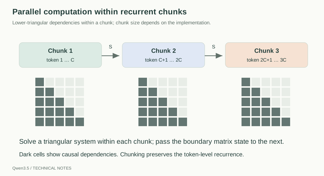
The source supplies both recurrent and chunked forms. Single-token decoding with an existing state uses the recurrent path; multi-token prefill or continuation uses the chunked path. The reference fallback defaults to chunk_size=64, while the fused kernel’s details depend on the backend. S1

Chunking reorganizes the same recurrence. It does not introduce future information or approximate the operation with unrestricted attention. Causal dependencies within a chunk can be expressed as a unit lower-triangular linear system. Matrix operations handle the chunk internally, and a matrix state connects consecutive chunks.

Given initial chunk state $S_0$, define:

$$d_i=\prod_{r=1}^{i}\alpha_r,\qquad R_{ij}=\begin{cases}d_i/d_j,&j\le i,\\0,&j>i.\end{cases}$$

Stack the keys, queries, and values as rows of $K,Q,V$. Let $B=\operatorname{diag}(\beta)$ and $D=\operatorname{diag}(d)$, and define the unit lower-triangular matrix:

$$A=I+\operatorname{tril}\big((BKK^T)\odot R,-1\big).$$

First solve:

$$U=A^{-1}BV,\qquad W=A^{-1}BDK,$$

then recover all correction vectors within the chunk:

$$\Delta=U-WS_0.$$

The outputs and final state are:

$$O=DQS_0+\big((QK^T)\odot R\big)\Delta,$$ $$S_{\rm out}=d_C S_0+ K^T\operatorname{diag}(d_C/d_j)\Delta.$$

The inverse notation expresses the mathematics; the implementation uses operations such as triangular solves rather than explicitly constructing a general matrix inverse. It also computes relative decay through differences of accumulated log-decays, avoiding division of two very small cumulative products. These equations explain why the implementation contains chunk-local Q @ K.T, accumulated decay, and lower-triangular solves while still avoiding an attention matrix of size $L\times L$ for the full sequence. S1

9.12 What fixed state buys, and what it loses

A DeltaNet head’s state does not grow with the number of past tokens, allowing recurrent processing with a fixed state size. That matrix cannot preserve an arbitrary history losslessly. Memory quality depends on how distinguishable the keys are, interference, gates, the training distribution, and what later queries ask for.

An architectural interpretation is that periodically inserted Full Attention layers preserve an explicit content-addressing path to past token representations, while linear layers reduce the cost of long context across much of the stack. This is a reasonable reading of the structure, not evidence from a hybrid-ratio ablation conducted in this article.

10. Full Attention: GQA, QK-Norm, and output gating

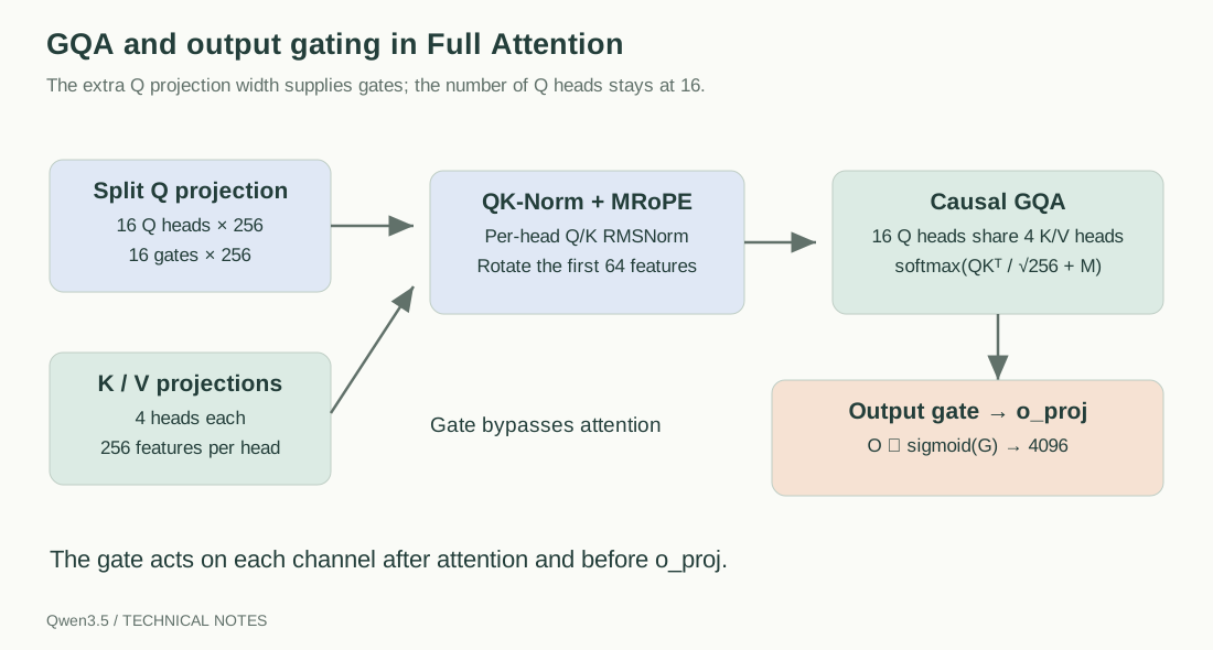
10.1 Why the Q projection is twice as wide

The 9B Full Attention layers define:

q_proj: 4096 -> 16 * 256 * 2 = 8192
k_proj: 4096 ->  4 * 256     = 1024
v_proj: 4096 ->  4 * 256     = 1024
o_proj: 16 * 256 = 4096 -> 4096

The extra width supplies an output gate for each head; there are still 16 Q heads. The source reshapes the projection to [B,L,16,512], then splits the final dimension into 256 dimensions for Q and 256 for the gate. Dividing a flattened 8192-dimensional vector into two contiguous halves would not necessarily preserve that channel layout. S1

10.2 Attention computation

Q/K first receive RMSNorm over their full 256-dimensional heads. Multimodal rotary encoding then rotates their first 64 dimensions. V is not rotated. Four KV heads support 16 Q heads, with each group of four query heads sharing one set of K/V; this is GQA. S1, C1

$$P=\operatorname{softmax}\left(\frac{QK^T}{\sqrt{256}}+M\right), \qquad O=PV.$$

$M$ includes causality and any required padding or sequence-boundary constraints. The output is flattened to [B,L,4096], then transformed as:

$$Y=W_o\big(O\odot\sigma(G)\big).$$

The gate acts elementwise on the attention output, before o_proj. It is not a factor inside softmax and is not one scalar shared across the sequence. S1

10.3 Comparing the two mixers

Property	Gated DeltaNet	Full Attention
Stored history	Recurrent matrix and local convolution state	K/V for each past token
Update	Decay, predict at the current key, write the error	Append K/V; queries address historical content
Softmax	Absent from the state update	Used in attention
Direct application of language RoPE	Absent on the inspected path	Applied to the first 64 of 256 dimensions
Q/K normalization	L2 normalization	Learned RMSNorm
Output gate	SiLU(z) after RMSNorm	sigmoid(G) on the attention output
History-state growth during ordinary decoding	Fixed size	Grows with sequence length

Source: S1. These entries describe the inspected implementation, not every model with a similar name.

11. MRoPE: three coordinates and a separate causal structure

11.1 Text and visual positions in one sequence

MRoPE assigns each token three coordinates, $(t,h,w)$. For text, all three are usually equal, copying a one-dimensional sequence position onto three axes. Visual tokens receive coordinates according to their temporal block and two-dimensional spatial grid. S1

These coordinates determine rotary phases. They do not directly determine which tokens can see each other. Actual sequence order, masks, and recurrence rules determine causality. Giving two visual tokens the same T coordinate does not make them bidirectionally visible in the language layers.

11.2 Partial RoPE rotates 64 of 256 dimensions

With head_dim=256 and partial_rotary_factor=0.25:

$$d_{\rm rotary}=256\times0.25=64.$$

Q/K are split into:

q_rot / k_rot:   first 64 dimensions
q_pass / k_pass: remaining 192 dimensions

Only the first part undergoes rotate_half + cos/sin, after which it is concatenated with the unrotated 192 dimensions. The latter remain in the attention dot product; they are not discarded. S1, C1

There are 32 base frequencies:

$$\omega_j=\theta^{-2j/64},\qquad j=0,\ldots,31.$$

11.3 The interleaved frequency layout

mrope_section=[11,11,10] allocates the 32 frequency positions to T/H/W in counts of 11/11/10. The source initializes from T, then overwrites H and W positions at a stride of three. S1

frequency index: 0 1 2 3 4 5 ... 27 28 29 30 31
axis:            T H W T H W ...  T  H  W  T  H

Specifically, T uses indices 0, 3, …, 30; H uses 1, 4, …, 31; W uses 2, 5, …, 29. A length-32 array does not continue to indices 33 or 36.

For frequency $j$, after choosing axis $a(j)$, the phase is:

$$\phi_j=\operatorname{pos}_{a(j)}\,\omega_j.$$

The 32 phases are duplicated into 64 dimensions according to the rotation layout, producing cos/sin. Interleaving chooses which coordinate axis supplies each frequency channel. It does not concatenate three separate attention outputs.

11.4 A complete image-position example

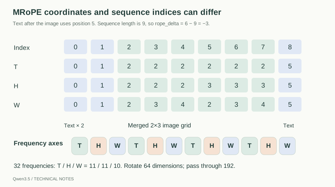
To make the arithmetic explicit, temporarily omit real chat boundaries. Consider two text tokens, an image with a merged 2×3 grid of six tokens, then one text token. The raw image grid is [1,4,6], with merge factor 2.

sequence index: 0 1 | 2 3 4 5 6 7 | 8
token type:     T T | I I I I I I | T
MRoPE T axis:   0 1 | 2 2 2 2 2 2 | 5
MRoPE H axis:   0 1 | 2 2 2 3 3 3 | 5
MRoPE W axis:   0 1 | 2 3 4 2 3 4 | 5

The image starts at position base 2 and reaches spatial coordinate 4. The next text position is therefore 5, although its physical sequence index is 8. The image occupies six tokens, but advances the position base by only $\max(2,3)=3$. That is the role of current_pos += max(grid_h, grid_w) // merge_size in get_rope_index. S1

This sequence has length 9 and a maximum rotary position of 5, giving:

$$\text{rope\_delta}=(5+1)-9=-3.$$

The next generated token has sequence index 9 and should use rotary position $9-3=6$. rope_deltas preserves this difference; three tokens have not gone missing. In padded batches, positions must also account for valid text positions rather than blindly using the total padded length.

11.5 Video timestamps and the T coordinate

Qwen3.5 represents video as repeated timestamp text followed by a visual segment. To match this structure, get_rope_index expands [T_g,H_g,W_g] into $T_g$ copies of [1,H_g,W_g]. S1, S6

The relative temporal coordinate within each visual segment is then 0, with the segment’s sequence position base added to it. Global T coordinates are not all zero. Timestamp and boundary text between adjacent segments also advance the position base.

Physical seconds, the temporal-group index, and the rotary T coordinate are thus different quantities. Time 3.5 seconds in a video does not directly imply RoPE T=3.5. Editing timestamp text does not automatically convert every rotary coordinate into the corresponding number of seconds.

11.6 Why position_ids can have three or four axes

get_rope_index returns T/H/W with shape [3,B,L]. Some generation-preparation paths retain ordinary text or sequence positions as well, concatenating them into [4,B,L]:

axis 0: ordinary text/sequence positions for masking bookkeeping
axis 1: multimodal T
axis 2: multimodal H
axis 3: multimodal W

TextModel uses the first axis for mask-related processing and sends the remaining three to the rotary module. The extra axis is neither a new spatial dimension nor a fourth independent attention mechanism. S1

11.7 Order sensitivity in DeltaNet without RoPE

The inspected DeltaNet forward does not directly apply position_embeddings. Its causal Conv1d and recurrence already depend on input order, however, and reordering tokens generally changes the state at each step. Hidden states that have passed through Full Attention also carry positional effects into later linear layers. S1

DeltaNet therefore remains order-sensitive without directly applying RoPE. Its recurrent state evolves along the actual input sequence.

12. Attention masks, causality, and training visibility

12.1 Three distinct causal structures

Vision ViT attention is noncausal spatial attention within a temporal group. Language Full Attention is causal attention over the fused sequence. Language DeltaNet obtains its ordered dependence from causal convolution and recurrence, without constructing a conventional softmax triangular attention matrix. S1, S7

TextModel therefore maintains separate full_attention and linear_attention masks. Full attention uses create_causal_mask; the linear layers use another helper:

create_recurrent_attention_mask(...)

A two-dimensional attention_mask input does not mean all layers ultimately perform the same two-dimensional masked computation. S1

Teacher forcing can supply a complete sequence in one parallel forward pass while still preventing a token from accessing future answers. Parallel execution is valid because the causal constraints remain in place. Chunked computation must preserve the same semantics.

12.2 Packed sequences require state boundaries

Packing several training samples into one long sequence requires more than preventing Full Attention from crossing sample boundaries. DeltaNet’s convolution and recurrent states must also stop at those boundaries. The source can pass information such as cu_seq_lens_q to a kernel, but the required reset behavior must be verified in the actual fused backend, fallback, and training framework. S1

An interface accepting attention_mask does not prove that arbitrary packing is correct. One useful check is to run two samples separately, then compare their outputs with the corresponding outputs of a packed run using declared boundaries. The check should cover ordinary attention, convolution state, and recurrent state.

13. Hybrid cache: prefill and token-by-token decoding

13.1 Two types of history in one cache

TextModel can create a DynamicCache from the configuration, but its contents depend on each layer’s type. Full Attention appends K/V; DeltaNet manages its state through update_conv_state and update_recurrent_state. S1, S8

For the ordinary 9B generation path:

Layer type	Persistent state shape per layer
Full Attention	K and V each [B,4,L,256]
Gated DeltaNet	Recurrent state [B,32,128,128]
Gated DeltaNet	Convolution state [B,8192,4]

A convolution kernel of size 4 makes the current output depend on four recent positions, three of which are in the past. Nevertheless, LinearAttentionLayer allocates its actual cache tensor with a final dimension of 4. Replacing it with 3 on the basis of the mathematical dependency would disregard the implementation’s state-management convention. S8

13.2 Prefill

Prefill processes the complete prompt. The vision encoder produces the required visual features, which are fused with text before entering the hybrid backbone. Full Attention performs causal prompt computation and stores K/V. DeltaNet processes the prompt in chunks and retains the final matrix and convolution states. S1

This cache contains more than one vector from the final layer. Each relevant decoder layer maintains its own history, and the states of different layers are not interchangeable.

13.3 Decode

With an existing cache and one new token, each linear layer updates its local convolution state and performs one recurrent delta-rule step. Each full-attention layer projects the current Q/K/V, appends K/V, and uses Q to read the cache positions allowed at that step. S1

Continuation should supply only tokens that have not already been processed, with the attention mask and position offsets maintained correctly. Sending the entire old prompt into the same nonempty cache counts that history twice and changes the result.

High-level generate handles much of this bookkeeping. A custom decoding loop must manage the range of new tokens, already consumed visual inputs, per-layer caches, effective sequence lengths, and MRoPE offsets. Merely retaining a variable named past_key_values does not implement the entire protocol.

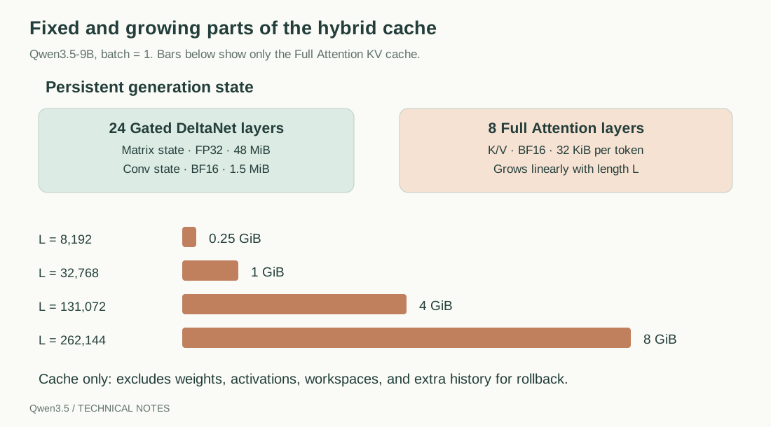
13.4 Memory calculations for 9B with batch size 1

The following counts only ordinary generation state. It excludes model parameters, activations, workspaces, communication, graph-capture preallocation, and additional history retained for rollback.

Each DeltaNet layer’s matrix state contains:

$$32\times128\times128=524288\ \text{elements}.$$

At float32, that is 2 MiB per layer, or 48 MiB across 24 layers. If the convolution state uses BF16, its total is:

$$24\times8192\times4\times2\ \text{bytes}=1.5\ \text{MiB}.$$

The total Full Attention K/V storage is:

$$8\times2\times4\times L\times256\times2 =32768L\ \text{bytes}.$$

Each additional token therefore adds 32 KiB of BF16 K/V across these eight layers alone. The total is 1 GiB at $L=32768$ and 8 GiB at $L=262144$.

Fixed-size linear-layer states do not give the whole model constant memory. Relative to 32 full-attention layers with the same head configuration, the number of layers storing K/V is reduced to one quarter. That does not prove that total model memory, measured latency, or training FLOPs also fall to one quarter.

13.5 Forking, rollback, and speculative decoding

Paths involving record_past change some storage decisions to retain additional information for rollback. The fixed-state estimates above explicitly exclude that mode. S8

Forking generation from an earlier position requires the Full Attention K/V and every linear layer’s recurrent and convolution states, together with position metadata. Truncating K/V alone cannot rewind a DeltaNet state that has already processed later tokens. Correct rollback needs snapshots, replay, or state management explicitly provided by the inference engine.

14. MoE: executing the sparse FFN in 35B-A3B

14.1 Its relation to the dense backbone

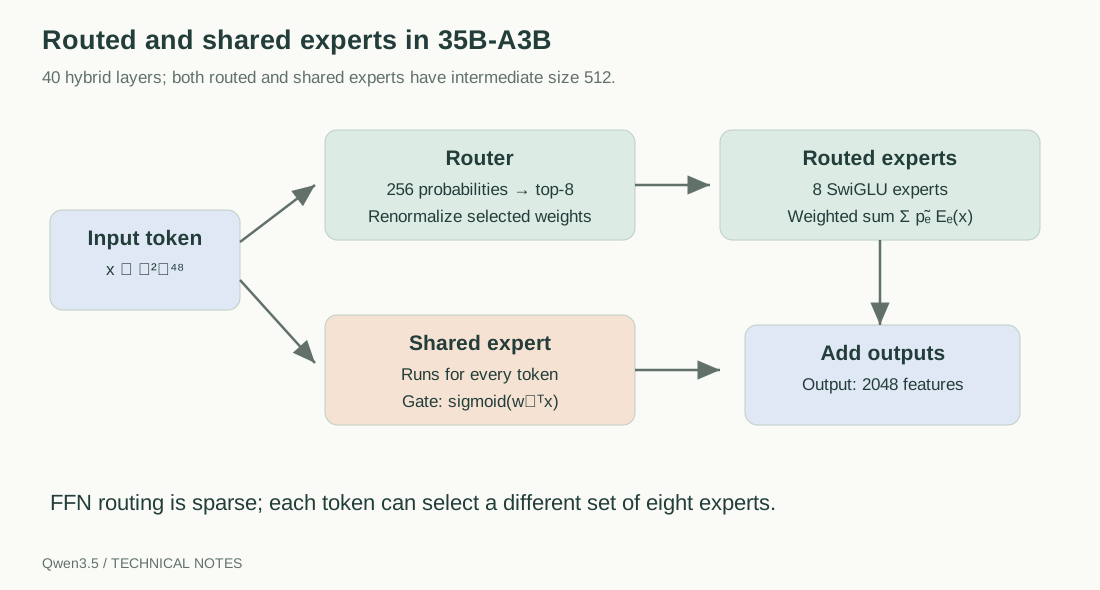
35B-A3B retains the same types of hybrid token mixers. Its 40 layers follow the 3:1 pattern, giving 30 DeltaNet and 10 Full Attention layers. Major structural differences include an MoE FFN in each layer and a text width of 2048. S9, C5

There are 256 routed experts, of which each token selects 8. Every expert has a SwiGLU intermediate size of 512. A separate shared expert also has intermediate size 512. This shared path does not participate in routing among the 256 experts.

14.2 Routing: softmax, top-k, and renormalization

Flatten the input to $X\in\mathbb R^{BL\times D}$. The router first computes:

$$r=XW_r^T,\qquad p=\operatorname{softmax}(r).$$

Softmax runs in float32 over all 256 experts. The router then selects the top-8 set $\mathcal K(x)$ and renormalizes the selected probabilities:

$$\tilde p_e=\frac{p_e}{\sum_{j\in\mathcal K(x)}p_j}.$$

The routed output for each token is:

$$y_{\rm routed}=\sum_{e\in\mathcal K(x)}\tilde p_e E_e(x).$$

Top-k selects FFN experts here, not attention heads, video frames, or input tokens. S9

14.3 The shared expert

The shared expert runs for every token and has its own sigmoid gate:

$$y_{\rm shared}=\sigma(w_s^Tx)E_s(x),$$

The outputs are added:

$$y=y_{\rm routed}+y_{\rm shared}.$$

The shared-path gate is one scalar per token, broadcast across the entire shared-expert output vector. It differs from Full Attention’s channelwise output gate. S9

14.4 Dispatch and combine in the source

Expert weights are stored as stacked tensors:

experts.gate_up_proj: [256, 2*512, 2048]
experts.down_proj:    [256, 2048, 512]

Conceptually, dispatch gathers the tokens selected for an expert, evaluates its SwiGLU, multiplies by routing weights, and accumulates the result into the original token positions through operations such as index_add_. The MoE’s input and output remain [B,L,2048]; it does not permanently split the sequence into 256 sequences. S9

Different tokens can choose different sets of eight experts. Across a batch, many or even all experts may be accessed. The active-parameter count in the model name therefore does not specify how many weights must be stored. Memory, expert parallelism, and communication also depend on deployment choices.

14.5 What inference code cannot tell us about training

The presence of router_aux_loss_coef shows that the public interface includes a parameter related to routing auxiliary loss. That field alone cannot reconstruct every load-balancing method, data mixture, optimizer setting, training stage, or effective loss used during pretraining. An inference architecture and a complete training recipe require different evidence.

15. From hidden states to answers: logits, loss, thinking, and MTP

15.1 The final LM head

After the last decoder layer, text RMSNorm yields [B,L,4096]. The LM head maps those hidden states to the vocabulary:

$$Z=HW_{\rm vocab}^T,\qquad Z\in\mathbb R^{B\times L\times248320}.$$

At the final position, softmax gives the conditional distribution of the next token. The 9B embedding and LM head use separate weights, while 4B ties them. Parameter estimates cannot count two independent matrices for both models. S1, C1, C4

15.2 logits_to_keep reduces head computation

Ordinary generation usually needs logits only at the last position. This implementation provides logits_to_keep: integer 0 keeps all positions, while 1 applies the vocabulary projection only to the final hidden state. S1

A long prompt therefore need not always materialize the full [B,L,248320] logits tensor. The prompt still passes through the language backbone to construct its attention caches and recurrent states.

15.3 Next-token alignment in supervised training

The outer forward accepts labels and passes logits and labels to the loss function. A typical autoregressive supervision objective is:

$$\mathcal L=-\frac1{|\Omega|} \sum_{t\in\Omega}\log p_\theta(x_{t+1}\mid x_{\le t}),$$

where $\Omega$ includes only supervised positions. The alignment is essential: logits at position $t$ evaluate the target at position $t+1$, not the input token already supplied at the current position.

The training data and collator are responsible for assigning -100 to ignored targets. In ordinary answer supervision, the user question, image placeholders, and unsupervised template portions should be masked according to the task protocol. The model’s forward pass should not be assumed to identify and supervise only the assistant answer automatically. S1

For an answer $y_1,\ldots,y_T$, the token log-probabilities sum to:

$$\log p_\theta(y\mid x)=\sum_{t=1}^{T} \log p_\theta(y_t\mid x,y_{<t}).$$

This is the log-probability of the sequence. Dividing by length produces a length-normalized score, which must be distinguished from the original sequence log-probability. Visual input changes these conditional distributions through the complete vision encoder, multimodal fusion, and hybrid decoder. There is no direct vocabulary softmax over pixels.

15.4 Backpropagation through the hybrid structure

In the dense model, supervised loss can propagate through the LM head, decoder layers, merger, and vision encoder. Which parameters update depends on what has been frozen. DeltaNet’s state update consists of differentiable operations and can receive gradients during training. Efficient implementations reorganize the calculation without removing the state update from learning.

For training across chunks, the training loop determines whether state gradients are retained, detached, or truncated. Ordinary generation caches use inference optimizations such as in-place updates and should not be taken as an implementation of full cross-chunk BPTT without inspection. Conventional full-sequence supervised training should generally disable inference caching and coordinate that choice with gradient checkpointing and other training settings. Cross-chunk training requires an explicit state and gradient protocol. S1, S8

15.5 Thinking mode uses the same decoder

The 9B chat template supports enable_thinking. When enabled, the generation prefix directs output into a <think> region. When disabled, the template supplies an empty think segment before the answer. Both modes use the same public backbone; there is no switch to a separate attention mechanism dedicated to thinking. C6

Generated thought tokens change subsequent layer states and K/V just as other autoregressive tokens do. One interpretation is that they can carry explicit intermediate computation or state descriptions. The appearance of think tags alone does not establish that the model executed any particular internal reasoning algorithm.

Tool calls in the template are likewise a structured text protocol. Executing tools, handling their results, and preparing the next input require an external runtime. The VLM forward pass does not itself operate the external environment. C6

15.6 MTP fields and the standard generation path

The 9B configuration includes fields such as mtp_num_hidden_layers=1. However, the standard generation-class forward inspected here connects the backbone to an ordinary LM head, and the pretrained model class includes rules for ignoring additional mtp.* loading keys. S1, C1

Configuration fields alone therefore do not show that ordinary Transformers generation automatically enables MTP acceleration, nor do they reconstruct the full MTP training objective. Checkpoint metadata, branches actually executed by the standard forward, and speculative or MTP support in a particular inference engine must be distinguished.

16. End-to-end tensor shapes

16.1 One 448×448 image

Assume the image already satisfies the processor’s size requirements. Let $L_{\rm other}$ be the actual tokenized count of all non-image-pad positions, including the question, template, and visual boundary markers.

Stage	Shape or count
Original RGB image	[3,448,448]
Grid	[1,28,28]
Preprocessed pixel patches	[784,1536]
Patch embedding	[784,1152]
Final output of 27 vision blocks	[784,1152]
Groups of four concatenated patches	[196,4608]
Merger output	[196,4096]
Image placeholders	196
Fused language input	[1,L_other+196,4096]
Each decoder output	[1,L_other+196,4096]
All logits	[1,L_other+196,248320]
Final-position logits only	[1,1,248320]

If, for illustration, the nonvisual portion tokenizes to exactly 64 tokens, the language sequence length is 260. That is an assumption for explaining shapes, not a measured token count for a particular Chinese prompt.

The input passes through DeltaNet layers 0, 1, and 2, followed by Full Attention layer 3, with this cycle repeated eight times. Image tokens remain part of later layers; they are not processed once in a dedicated visual decoder layer and then set aside.

16.2 One image, eight video frames, and text

Assume the image and every video frame are 448×448, and the video contains the eight sampled frames described earlier:

image pixels:          [784, 1536]
image_grid_thw:        [[1, 28, 28]]
image merged features: [196, 4096]

video pixels:          [3136, 1536]
video_grid_thw:        [[4, 28, 28]]
video merged features: [784, 4096]

total visual tokens:   196 + 784 = 980
language sequence:     980 + all other token positions

The outer forward processes images and videos separately, then scatters their features into the actual corresponding placeholder positions. Sharing one vision encoder does not mean that this outer call necessarily concatenates both modalities into one vision forward batch. S1

For the video, ViT cu_seqlens is [0,784,1568,2352,3136]; for the image it is [0,784]. The language layers subsequently process the combined sequence.

If the other tokens total 64, again as an assumption, then $L=1044$. The first DeltaNet layer has the following shapes:

hidden states:      [1, 1044, 4096]
projected QKV:      [1, 1044, 8192]
causal conv input:  [1, 8192, 1044]
Q/K before repeat: [1, 1044, 16, 128]
Q/K after repeat:  [1, 1044, 32, 128]
V and z:           [1, 1044, 32, 128]
a / b:             [1, 1044, 32]
final state:       [1, 32, 128, 128]
output:            [1, 1044, 4096]

The first Full Attention layer uses:

Q:             [1, 16, 1044, 256]
K/V:           [1, 4, 1044, 256]
RoPE cos/sin:  [1, 1044, 64]
attention out: [1, 1044, 4096]

After GQA expansion, an eager implementation may form attention weights of shape [1,16,1044,1044]. Efficient Flash/SDPA paths need not materialize that complete matrix. Their attention semantics nevertheless remain different from DeltaNet’s recurrence.

17. Complexity and parameter counts

17.1 Cost of the visual front end

Let each temporal group contain $n=H_gW_g$ raw patches, with $T_g$ groups. The quadratic component of visual attention is approximately:

$$O(T_g n^2D_v),$$

rather than $O((T_gn)^2D_v)$ for unrestricted attention across all groups. Projections and MLPs still contribute substantial computation linear in token count. Increasing spatial resolution can sharply increase ViT cost, while reducing the temporal sampling rate primarily reduces the number of groups. S1, S7

The merger comes after all 27 ViT blocks. Using the already reduced visual token count to estimate those preceding attention operations would undercount their cost.

17.2 The hybrid language backbone is not globally linear in length

Ignoring constants from projections and FFNs, Full Attention prefill contains an $O(L^2)$ term. The DeltaNet state core is approximately $O(LH_vd_kd_v)$ in sequence length, with the chunked implementation organizing local quadratic work into fixed-size chunks. S1

The 9B stack substitutes DeltaNet for 24 layers and retains 8 Full Attention layers. The defensible conclusion is a substantial reduction in the number of full-attention layers and their KV costs, rather than strictly linear complexity for the entire model.

Actual speed also depends on FFNs, projections, the vision front end, kernels, parallelism, and hardware. Short sequences, Python/PyTorch fallback paths, or missing fused kernels can prevent a complexity advantage from becoming a wall-clock advantage. This article does not measure those speeds.

17.3 Counting the 9B visual front end analytically

The following counts use the 9B configuration and inspected module definitions, including the relevant biases and normalization parameters. They do not load actual weights and exclude MTP and additional modules outside the standard forward path.

Module	Parameters
Patch embedding	1,770,624
Learned visual position table	2,654,208
Attention in each vision block	5,313,024
MLP in each vision block	9,921,872
Two LayerNorms in each vision block	4,608
Final merger	40,119,040
Total for 27 blocks and the input/output modules	456,010,480

For example, patch embedding contributes $3\times2\times16^2\times1152+1152$ parameters. The two visual MLP matrices and their biases contribute $2\times1152\times4304+4304+1152$. Such explicit expressions are easier to verify than a version-independent claim that the vision encoder has “about 300M” parameters.

Under the same counting convention, the 9B text backbone and separate LM head have 8,953,803,264 parameters. Adding the visual front end gives 9,409,813,744. This is an analytical count of standard modules built from the inspected configuration, not an inventory of checkpoint contents, MTP weights, or actual resident memory.

References

S1 Dense model forward implementation.

S2 Qwen3.5 configuration classes.

S3 Dense model modular source.

S4 Image preprocessing implementation.

S5 Video preprocessing implementation.

S6 Unified processor, timestamps, and placeholders.

S7 Visual grids, interpolation, and attention-segment helpers.

S8 Cache types and linear-state management.

S9 MoE model forward implementation.

S10 MoE modular inheritance.

C1 Qwen3.5-9B checkpoint configuration.

C2 9B image processor configuration.

C3 9B video processor configuration.

C4 Qwen3.5-4B checkpoint configuration.

C5 Qwen3.5-35B-A3B checkpoint configuration.

C6 9B chat template.

P1 Gated Delta Networks paper.